
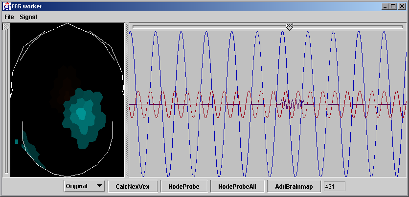
The display of the fake signal from one of the weakest nodes.
This page follows on from the Step-by-step guide.
When you have the example fully loaded, it is necessary to clear it. Select File | ResetAllVex from the menu-bar to clear everything from the Brain Patterns window. Now select Signal | Clear from the menu-bar to clear all the data.
You can load up the first, second or third experiments from the sample data by selecting Add Signal 0, Add Signal 1 or Add Signal 2 respectively. You can get an average of the three signals by selecting Add All Signals. If you have a few more than just the three in your data set, this is a good way to see the evoked potential response, I am told.
Please clear the data again and select Add Fake Signal.
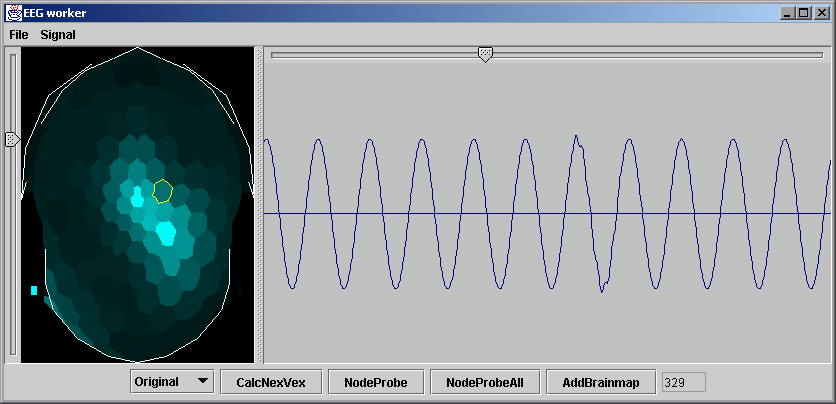
The picture shows that you have the sum of three different oscillating generators. The weak one in the middle is short, very tiny and hard to see, but its trace is shown here.
 |
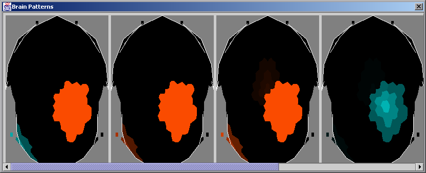
Do CalcNextVex a few times to get:
 |
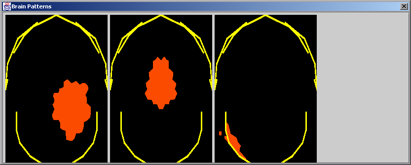
Doing NodeProbeAll seems to show up the the places where you can find the three generators.
 |
The EEG pattern given in the picture at the top is the sum of three independent generators. The patterns of these generators are fairly clear. They are composed of the highest signal on a central node, a two thirds signal on their neighbouring nodes, and a half signal on the neighbours of that. Everything else is zero. This is in fact the pattern we use for the node probe. What we do is try and make a combination of the patterns in the Brain Patterns window that most closely approximates the probed pattern. The probed pattern is not very important because it can't force combinations that are not already possible in the raw data. But better results might be obtained using a different probe pattern. One would need to program other ideas and experiment with them.
 |
 |
If you reset everything and have the fake signal loaded, you can select Signal | Add Noise from the menu-bar to get a noisy signal.
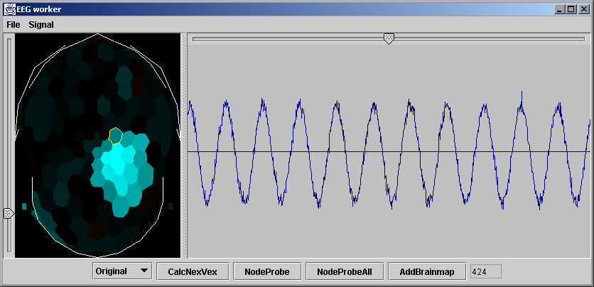 |
If you repeat the procedure of extracting the generators, you will find that the weakest signal is almost entirely lost. Had you not erased the saved brain patterns you got from the non-noisy signal, you could have stored them in the brain patterns window and found the weakest signal still there.
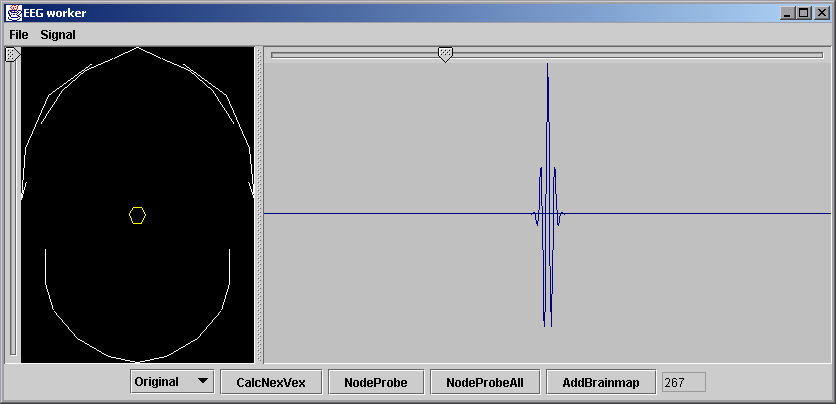
Also, I have included some preliminary work on wavelet transforms (a feature normally used from MatLab in spite of the fact that this program demonstrates how you can do without such expensive applications to get the job done). Select Signal | Clear followed by Signal | Add Wavelet, and select the central node as shown to get a look at the wavelet shape that is used in the next demonstration.
 |
To demonstrate the wavelet transform, select Signal | Clear followed by Signal | Add Fake Signal. Find the node in the middle with the tiny waveform signal. Select Signal | Add Noise which swamps it. Then select Signal | Wavelet Trans to once again bring the signal out.
A combination of well-chosen wavelet transforms (which is a linear transform on the data) to amplify certain generators, and reloading the original untransformed data as you build up the generators in the Brain Patterns window should, in theory, do as much as can be done with the data from the point of view of linear algebra.
I don't have time for any further development on this program, because it is not my job to be a psychologist, but I am more than happy to help anyone who wants to turn this into a serious application. Go back and visit the next page to get an overview of the structure of the program.